


Financial Stability Course
Mexico City, Mexico. 18 and 20 September 2019
This newly course focused on General Equilibrium and DSGE models for financial stability purposes. A second objective of this course is to provide visual and analytical financial stability tools including network analysis for financial stability analysis.
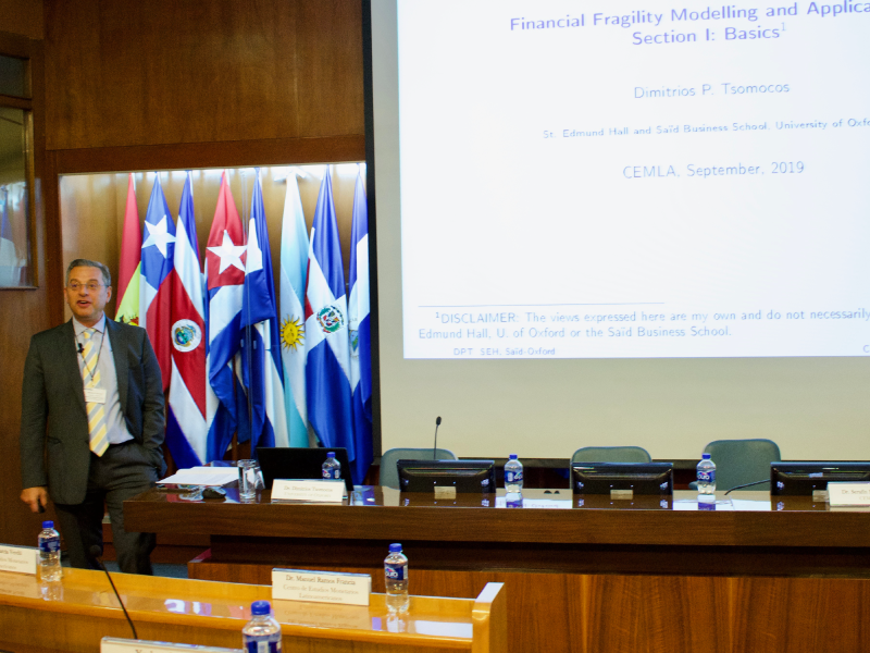
Modeling liquidity, default and financial stability in general equilibrium
Dimitrios Tsomocos
Professor Tsomocos organized his first session on the following topics: security markets, arbitrage pricing, state contingent prices and financial equilibrium. First, he explained how to model uncertainty and defined securities markets. Additionally, he identified some important definitions in the security markets context, as price, securities payoff and portfolios. He went on to define ‘complete markets’ and ‘incomplete markets’ and from there he introduced the Arrow-Debreu model in which equilibrium is equivalent to an asset equilibrium with complete markets. He also explained that the Arrow-Debreu equilibrium is Pareto Optimal (First Welfare Theorem), whereas the Financial Markets Equilibrium (which considers incomplete markets) is constrained suboptimal (Second Best). Other assumptions for the latter equilibrium are: the no existence of initial endowments and the no arbitrage property. The financial equilibrium is solved through the Kuhn-Tucker methodology, where the agents maximize their utility subject to their budget constraints and market clearing conditions (for goods and securities markets) to find an interior solution for prices.
Then, Professor Tsomocos focused on modeling default, which is costly for the creditor the debtor and for the market and is essential for financial stability analysis. He explained the implications of default when markets are incomplete as: i) the spanning property (provides extra insurance opportunities to the creditor), ii) allows the debtor to customize his own insurance opportunities; and iii) agents can be on both sides of the market (pooling). He explained that when default is allowed, the need to impose penalties arise; otherwise agents would default and no assets would be traded. Default is interesting only in incomplete markets. Thus, financial fragility is a result of a default general equilibrium phenomenon with incomplete markets and money. The principal elements to model default are: continuous penalties and the collateral as a cost reflected on margins. Collateral is assumed to be observable to avoid adverse selection issues.
Finally, he defined financial instability as any deviation from the optimal saving-investment plan of an economy that is due to imperfections in the financial sector. Generally, this is accompanied by a decrease in economic welfare. He highlighted that the principal differences between price stability and financial stability consists of the measurement, instrument for control and the forecasting structure. For instance, financial stability focuses on the tails of distribution, while the price stability employs the central moments of the distribution.
An Integrated Framework for Analyzing Multiple Financial Regulations
Dimitrios Tsomocos
In this session Professor Tsomocos presented a model that studies the externalities that emerge from intermediation and examined regulation to mitigate their effects. This model is based on the classic Diamond-Dybvig model with some modifications. There are three players in the model, the entrepreneurs, savers, and the bankers. Banks provide liquidity and monitoring services; are funded by deposits and equity; make risky loans; hold liquidity and are subject to limited liability; and face endogenous run risk determined by a global game.
The assumptions for this model are (i) the quasi-linear preferences for consumption and additional utility from the transaction’s services of deposits, (ii) the entrepreneurs are risk neutral and have no endowment of their own and (iii) the entrepreneurs have a linear production function, but incurs a convex (effort) cost. In the optimization problem the productivity shock is privately revealed to entrepreneurs, the banks need to spend resources to learn it. The bank monitors if the net expected benefit from monitoring is greater or equal to zero. If the bank does not monitor, the entrepreneurs will report the bad shock and default, and this will have implications for the global game.
To sum up, this model presented fragile financial intermediation where a bank offers liquidity and monitoring services. Also, this model studied the externalities from intermediation and derived optimal regulation to address them and proposed a new proof for uniqueness in incomplete information bank-run models. Some regulatory tools that work are the liquidity coverage ratio, the net-stable funding ratio, reserve requirements, and the leverage ratio. Professor Tsomocos pointed out that the minimum the regulator needs is a tool to manage capital, a tool to manage liquidity and a tool to manage the scale of intermediation. The liquidity tools can be combined with capital tools (and vice versa), but not with each other.
Financial stability analytics
Mark Flood
Professor Flood explained the different mechanisms of systemic risk build up: global imbalances, correlated exposures, spillovers to the real economy, information disruptions, feedback behavior, asset bubbles, contagion and negative externalities. Mr. Flood pointed out the statistical challenges, as the “maginot” problem which explains that a single measure is not sufficient.
Mr. Flood presented the trends in credit intermediation from 1952 to 2017 and the increased evolution of mutual funds, securitization, repo, commercial paper, the rise of fintech intermediaries and others. Flood pointed out that big data is a scalability problem with the following implementation challenges: volume, velocity and variety. For financial stability monitoring with big data, Flood et al. (2016) suggested a five tasks procedure that consist on data acquisition, data cleaning, data integration and representation, data modeling and analysis, and data sharing and transparency. For example, in data integration is important to introduced the global legal entity identifier (LEI) to minimize confusion among entities and the information could be standardized.
The fundamental rule of data collection is the standardization of data. Finally, Mr. Flood suggested an interesting list of readings and sources to read more about this topic.
Data visualization and financial stability
Mark Flood
The core functions of visualization consist on sensemaking, decision-making, rulemaking, and transparency. According to Shneiderman (1996), there are seven data types of interactive visualization: one-dimensional, two-dimensional, three-dimensional, temporal, multidimensional, tree, and network. For each type, Mr. Flood explained with examples the usage and the differences for each interactive visualization and their importance for decision-making using time series data.
Finally, Mr. Flood explained deeply the visual analytics by explaining the analytical reasoning of visual interfaces, the different levels of human perception and it representing relationships. Also, the details for exploiting human perception, the features with visual salience as color contrast, the visual salience failure, texture recognition, contour recognition, Gestalt perception, lightness and brightness; optimizing the “signal-to-noise” ratio in the visualizations, for example increasing the volume of “ink” according with the importance of the element.
Liquidity and default in an exchange economy
Dimitrios Tsomocos
Professor Tsomocos presented a model of trade and intermediation that allows the authors to study financial stability under the presence of financial frictions (liquidity and default). With the theoretical and empirical evidence of the interplay of liquidity and default he built a framework that allowed him to explain the effects of liquidity and default on welfare and financial stability. He explained that the default and liquidity frictions are sufficient to explain price and activity trade-offs. He explained a model that focuses on liquidity effects on financial stability.
The market structure of the model consisted of households, commodities market, commercial banks or asset markets, interbank markets and a central bank or a regulator which holds the open market operations and the default code (penalties). This latter is related to the financial frictions that consisted on default and money; they model the punishment in case of default with non-pecuniary penalty proportional to the defaulted amount of credits (households and commercial bank loans). Also, he highlighted the default choice trade-offs, on the one hand the benefit of defaulting, this means more consumption; and on the other hand, its cost (credit costs). Money is introduced by a cash-in-advance transaction technology and it is modeled as inside money. Liquidity has two sources, the first one through the injections by the Central Bank through open market operations and the second one by a fraction of the goods’ trades on every period that can be used immediately as a mean of payment.
Additional assumptions are that the only way to smooth consumption is through commodity trade, assuming a stochastic AR(1) process for the commodity endowments and an endowment economy. He presented the household optimization problem, the bank optimization problem, rational expectations and market clearing conditions (commodity, consumer loans, and repo market). From his model, he defined short-run financial stability with money, liquidity and default equilibrium if and only if all agents optimize given their budget sets, all markets clear and expectations are rational. In the long run the economy converges to its steady state. Also, he defined four propositions, the first one refers to the non-neutrality of money, this proposition implies that if there is a non-zero monetary operation by the Central Bank, monetary policy is not neutral in the short-run, thus, it affects the consumption and consequently real variables. When we have no liquidity restrictions, there are no incentives to borrow money and monetary policy is neutral, and in this case, default does not make sense, since there is nothing to default on. But, if there is full liquidity, the model would be a standard Edgeworth 2-agents 2-goods case. The second proposition refers to the Fisher effect; this proposition indicates that nominal interest rates are approximately equal to real interest rates plus expected inflation and risk premium, which depends on liquidity and default. The Fisher effect explains how nominal prices are linked directly to consumption. Proposition 3 refers to the quantity theory of money, where money supply has a direct, proportional relationship with the price level.
Finally, proposition 4 refers to the on the verge condition, which implies that the optimal amount of default is defined when the marginal utility of defaulting equals the marginal dis-utility. Lastly, Professor Tsomocos concluded that liquidity and default in equilibrium should be studied contemporaneously, the presence of financial frictions underlines the importance of studying the impact of shocks on the behavior of short to medium run of financial variables and welfare. In his model, he derived a relationship between prices and activity (trade) with the inclusion of default but without nominal frictions.
Debt, recovery rates and the Greek dilemma
Dimitrios Tsomocos
Professor Tsomocos explained with a model the Greek dilemma. First, the default is made synonymous with the restructuring of debt and he argued that immediate restructuring, reduces the present value of debt, and this would benefit both Greece as well as its creditor countries over the medium and long term. He described the framework of this model as a decentralized two-country RBC model, where Greece is the debtor nation and Germany the main creditor nation. The Greek households can issue both secured and unsecured debt to German households and the possibility of renegotiating on unsecured debt exists. The expectations of creditors determine whether a (good) default-free or (bad) default steady-state equilibrium prevails. Greeks may, at a cost, restructure or renegotiate unsecured debt and get a haircut. In this model, the authors explicitly modeled the decision to default, the default channel, which exacerbates the volatility of consumption, may be reduced with more lenient, but appropriate, debt restructuring terms. This means that the dilemma is not whether there is a moral duty of creditor nations to transfer resources to Greece, but whether creditors are willing to trade-off short-term losses for medium and long-run gains. Dr. Tsomocos explained the four claims related to credit conditions and debt restructuring: moral hazard matters, renegotiation costs are contingent on aggregate default rates, renegotiation is contingent on private-sector financial vulnerability and that renegotiation is contingent on economic activity and debt sustainability. With this claims the Greek households decide how much debt to renegotiate taking it into account; the creditors agree to reduce the present value of debt obligations by the “recovery rate”. Also, he explained the default accelerator term where the default is endogenous, depends on debt to capital (GDP proxy) ratio and depends on the amplification that default of individuals has on the propensity of others to default (banking system / balance sheet).
Finally, he concluded that this model, only examines the time-consistent path of debt agreements, the moral hazard aspect of debt is captured in the cost of reneging on contractual obligations. Lastly, he stressed that quantitative easing and debt monetization might increase discord among Eurozone member states due to the heterogeneity of the zone.
Stress testing and financial stability,
Mark Flood
In this session, Mr. Flood presented an overview of the different stress testing frameworks and give their characteristics and specific examples for each one. He also gave additional information about the next generation models which would be incorporating reaction functions, modeling systemic effects, shifting landscape, and incorporating agent-based modeling. He presented an optimal uncertainty quantification model which guarantees that the probability measure of system response is equal or greater to a specific threshold; this means that is the probability that some event occurs (typically undesirable). Additionally, he explained the different concentration inequalities: Chebyshev and MCDiarmid inequality. The principal components analysis consisted of extract from time series of daily bond price changes, where the first three components explain the 99.9977 percent. He pointed out that we have to take into account the heterogeneity in macroprudential stress testing because there are multiple transmission channels and multiple firms and sectors. Finally, he explained the importance of modeling heterogeneity and the need for multiple scenarios to achieve the systemic risk objective.
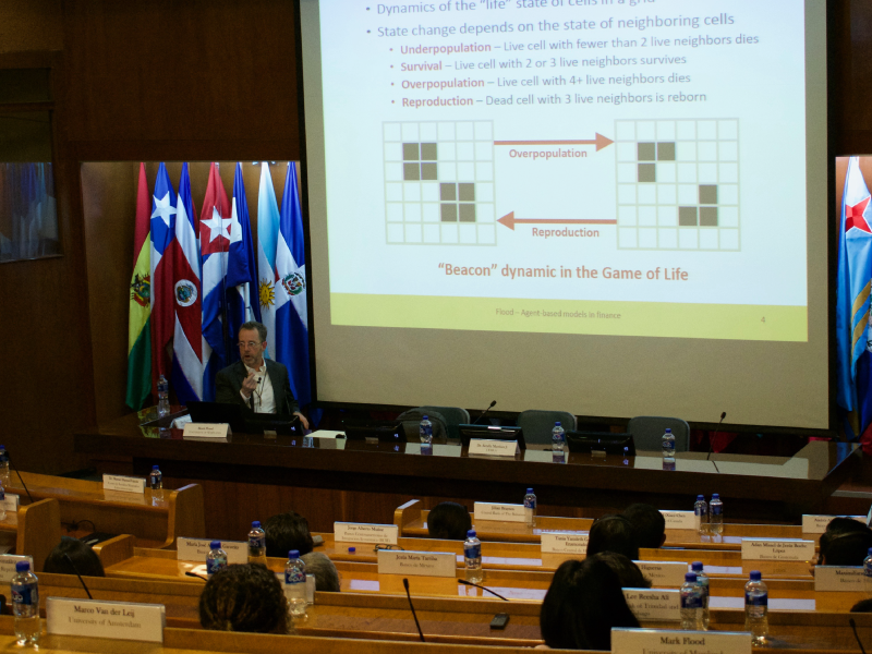
Agent-based modeling and market liquidity
Mark Flood
In this session Professor Flood presented the historical context for agent-based economics and defined the agent-based models (ABM) as a collection of agents, interacting to generate a system’s global behavior. The advantages of this type of modeling are that representative agent models overemphasize model tractability, whereas ABM, uses heuristics and bounded rationality instead. The agents-based models have different emphases from representative-agent models, for instance, they include heterogeneity, local interactions and systemic dynamics. However, there are challenges related to the robustness, estimation, and calibration because there is a lack of standards, a dependence on interaction model and the ecological inference that refers to drawing conclusions about individuals from aggregates. Additionally, he explained the reduced form heterogeneous agent models where the heterogeneous agents are from two behavioral categories, for example, informed vs noise, or fundamentalist vs chartist; and bounded rationality that frequently uses closed-form mathematical solutions.
Finally, Mr. Flood explained the basic framework for chartists and fundamentalists and a variety of examples as the destabilizing rational speculation, volatility clustering, and banking fire sales. Professor Flood pointed out the estimation methods through the maximum likelihood estimation, method of moments, latent variables, and Bayesian methods. Additionally, he described the implementation, in particular, object-oriented programming and the simulation tools for agent-based modeling, for example, Swarm (objective C, Java), NetLogo, Repast (Java), MASON (Java), AScape, MESA (Python) and HARK (Python).
General findings of the model, Calibration and Results. Chile Case study. Sovereign Credit Risk, Financial Fragility and Global Factors
Dimitrios Tsomocos
Professor Tsomocos continued his session with the Chilean Case study where the aim was to identify the impact of real and nominal shocks to financial stability for small open economies and commodity exporters. Professor Tsomocos developed a model for a small open economy to study financial stability, this model incorporates heterogeneity in the banking system. First, he explained the Chilean context and the economic characteristics that are important to understand the evolution and the trends of this economy as a result of an evolution to an open economy with a safe banking system. For instance, there is still dependence of copper process that may feedback to the financial sector directly or indirectly, the size of the impact depends on the country’s external position and bank heterogeneity have an important role in this model, that Professor Tsomocos explained later. This paper concerns macroprudential regulation/monitoring in fragility times with macroeconomic shocks being amplified due to the presence of pecuniary externalities. There are two sources of externalities, one is the cost of default and the other one the collateral constraints dependent on market valuation of capital. In this model the banking sector is perfectly competitive and there is ex post heterogeneity manifested on idiosyncratic shocks experienced by small banks. The assumptions for this model are the following: New-Keynesian DSGE model with nominal rigidities, commodity exporter small open economy, no barriers to trade, there is households, firms, external sector, Central Bank, Regulator and Government, heterogeneous two period lived firms with idiosyncratic risk and default, heterogeneous two period lived banks, and capital requirements, there is default for secured and collateralized loans and capital requirements.
Finally, Professor Tsomocos demonstrated that adverse shock to copper price significantly has both real and financial effects that reinforce each other, the default rates transmit the impact to interest on unsecured borrowing and reduces investment. With this model, it is possible to study the effect of shocks on monetary policy to financial stability.
A brief introduction to financial networks. Construction of financial networks from bilateral exposures and balance sheet data
Marco van der Leij
In this session, Professor van der Leij explained the two most basic financial network concepts: nodes and links. The first one refers to the financial institutions (banks), the second refers to the links between banks as exposures, common assets, funding. Financial contagion is built from the spread of a shock from one bank to other banks through the financial network. He also mentioned that systemic risk can be defined as the risk that financial stress in one bank leads to financial stress in the whole financial sector.
Professor van der Leij explained asset pricing and balance sheet approaches in financial networks. The asset pricing approach consists on publicly traded stock market process of banks and the network estimated from time series dependencies through methodologies such as SRISK and CoVAR. The balance sheet approach consists on private data taken from assets and liabilities of banks, where the network is partly known and the systemic risk is estimated from assumptions on contagion mechanism.
The main types of contagion channels are: default cascades, funding contagion, and the fire sales externality. The default cascades consist on a shock transmitted through assets side and it gets amplified by bankruptcy cost, incorporating default risk in the asset values and by fire sales externalities. While the shock in a funding contagion is transmitted through the liability side and gets amplified by liquidity hoarding and sales of illiquid assets (fire sales). Finally, the fire sales externalities are created from a shock on asset prices and which assumptions consist on illiquid assets, and that balanced sheet assets are valued at mark-to market. In this section, Professor van der Leij solved numeric exercises for each type of contagion model and explained other exercises applying the default algorithm of Eisenberg & Noe and the DebtRank algorithm and the comparison between both algorithms.
On the one hand, DebtRank is a dynamic algorithm process which is an upper bound on contagion or a contagion before default mechanism. On the other hand, Eisenberg-Noe consists of accounting identities, with a fixed-point clearing vector, which is a lower-bound on contagion, a contagion only after default and no contagion in quiet periods.
Professor van der Leij explained how to construct network data to analysis financial contagion from incomplete information: the information available is the one for large exposures, for certain registered type of transactions and for banks within own jurisdiction. We need to estimate networks using bank balance sheet reports (aggregate interbank assets and liabilities often available), available network data (large exposures) and with general information on financial network structures. Also, in the last part of the session, the group compute by hand the default algorithm of Eisenberg & Noe, and the DebtRank algorithm of Bardoscia, Battiston, Cacciolli et Cardarelli.
Finally, Professor van der Leij focused on the financial network structure and its estimation; he explained that their structure has the following common characteristics: relatively few links (low density), large inequality in number of links among banks, short path lengths, and a core-periphery structure. For the estimation, it is common the use of the Bayesian approach when we have information on aggregate interbank assets and liabilities, known links and some random network model, then we need information on the distribution of potential networks. The latter can be sampled from the distribution of potential networks using Gibbs-sampling with the systemicrisk package available in R.
Contagion channels in financial networks: default cascades, liquidity contagion, and asset fire sales. Quantification of systemic risk in banking networks
Marco van der Leij
In this session, Dr. van der Leij explained the typical characteristics of balance sheet data and large networks, constructed a financial network from balance sheet data and large exposures. Also, he computed metrics of financial contagion at system level and bank level. Finally, he explained the multilayer network and the importance of assessing systemic risk from Poledna et al. paper. In this paper, the authors considered data of different exposures between banks in Mexico, analyzed individual layers and the combined multilayer network using a systemic risk measure based on DebtRank methodology. They used daily bilateral exposures data on 43 banks in Mexico from 2007 to 2013: derivatives, securities, foreign exchange and deposits and loans.
The key findings of that paper were that the use of interbank loans and no other layer underestimates systemic risk by 90%; the systemic risk of the combined exposure network is higher than the sum of the four layers. The contribution of a credit transaction to expected systemic loss is up to a hundred times higher than the corresponding credit risk. To sum up, the financial markets underestimate current systemic risk.
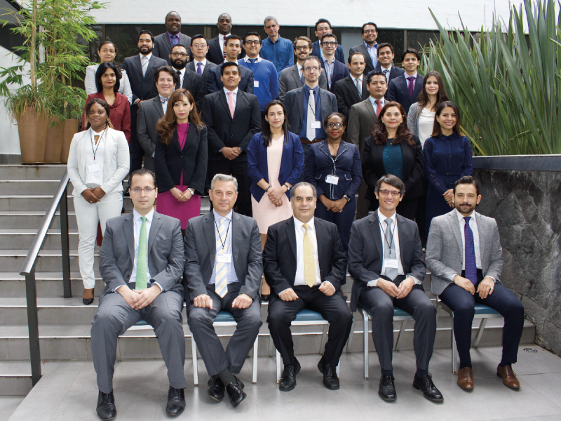
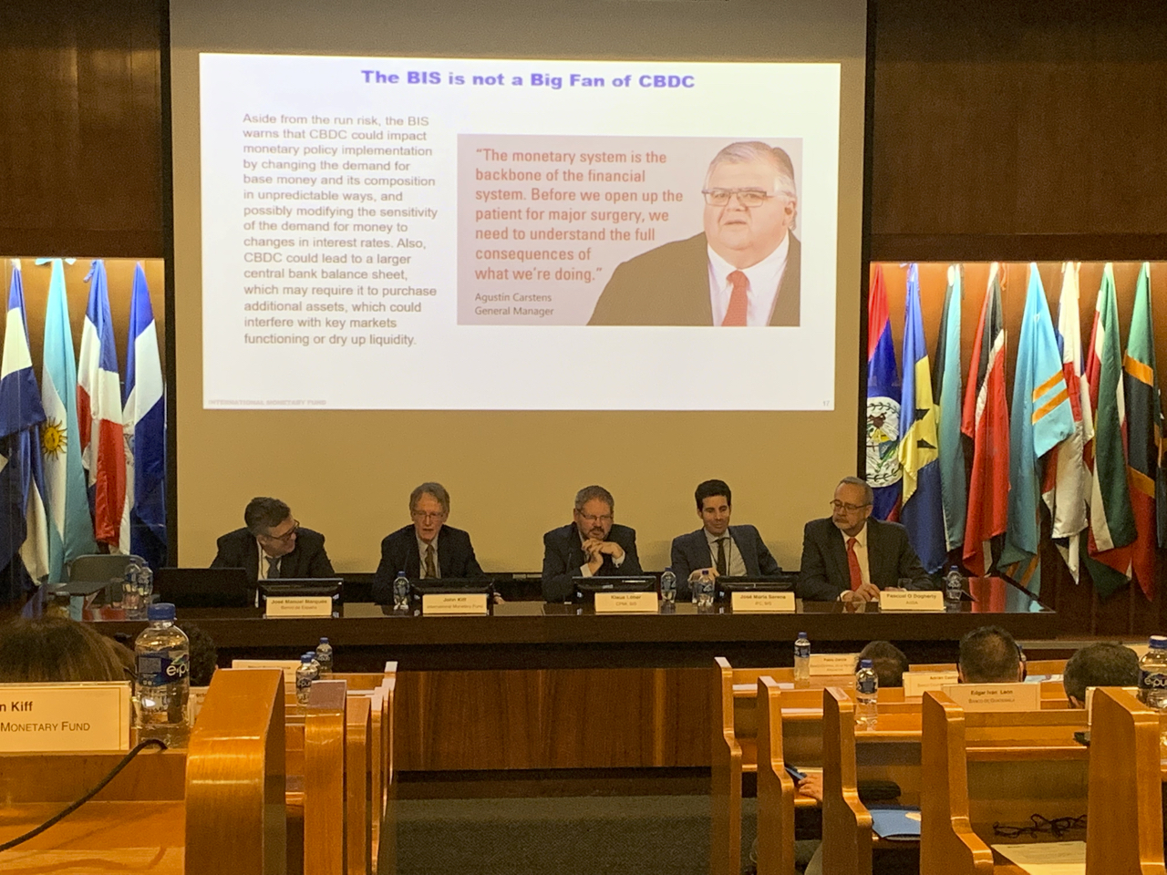
Day 1
Opening session ![]()
Dr. Serafín Martínez-Jaramillo, Advisor, CEMLA
Modeling liquidity, default and financial stability in general equilibrium ![]()
Dimitrios Tsomocos
An Integrated Framework for Analyzing Multiple Financial Regulations ![]()
Dimitrios Tsomocos
Financial stability analytics ![]()
Mark Flood
Data visualization and financial stability ![]()
Mark Flood
Day 2
Liquidity and default in an exchange economy ![]()
Dimitrios Tsomocos
Debt, recovery rates and the Greek dilemma ![]()
Dimitrios Tsomocos
Stress testing and financial stability ![]()
Mark Flood
Agent-based modeling and market liquidity ![]()
Mark Flood
Day 3
General findings of the model, Calibration and Results. Chile Case study ![]()
Dimitrios Tsomocos
Sovereign Credit Risk, Financial Fragility and Global Factors (Continuation) ![]()
Dimitrios Tsomocos
A brief introduction to financial networks ![]()
Marco van der Leij
Construction of financial networks from bilateral exposures and balance sheet data (Continuation)![]()
Marco van der Leij
Contagion channels in financial networks: default cascades, liquidity contagion and asset fire sales (Continuation)![]()
Marco van der Leij
Quantification of systemic risk in banking networks (Continuation) ![]()
Marco van der Leij
Closing, course evaluation and handing of certificates
Dr. Serafín Martínez-Jaramillo, Advisor, CEMLA
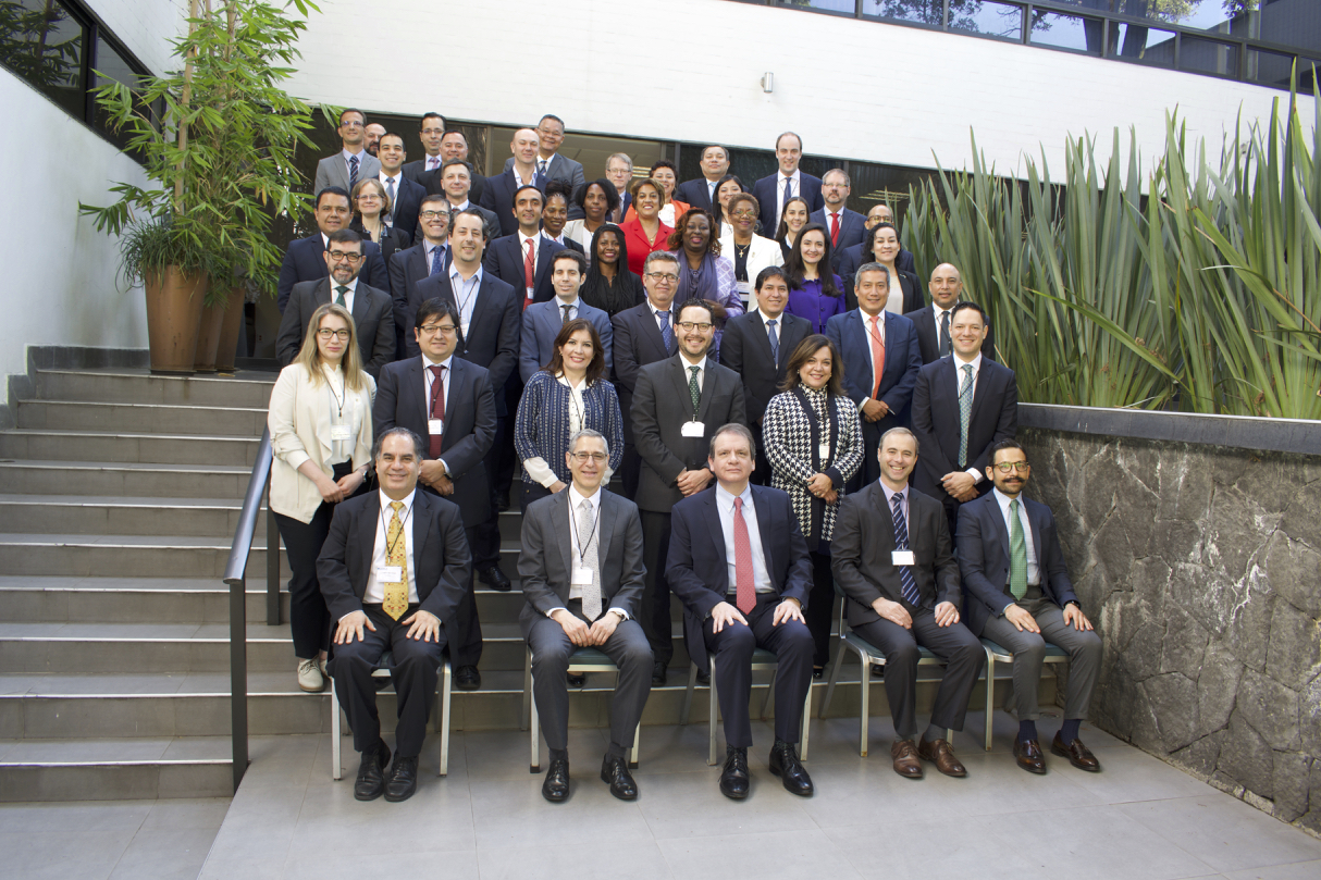
CEMLA has organized the first edition of Financial Stability Course with a distinguished group of experts from the academia who shared their perspectives and knowledge on financial stability. The Course has the aim to become a reference across the region and, more importantly, to contribute training CEMLA’s Membership with analytical capacity to better face new challenges in financial stability analysis and monitoring.
 Dr. Dimitrios P Tsomocos
Professor of Financial Economics at Saïd Business School and a Fellow in Management at St Edmund Hall, University of Oxford
Dr. Dimitrios P Tsomocos is a Professor of Financial Economics at Saïd Business School and a Fellow in Management at St Edmund Hall, University of Oxford. A mathematical economist by trade, his main areas of expertise include:
- Incomplete asset markets
- Systemic risk
- Financial instability
- Issues of new financial architecture
- Banking and regulation
Dimitrios' research has had a substantial impact on economic policy around the world. In particular, he analyses issues of contagion, financial fragility, interbank linkages and the impact of the Basel Accord and financial regulation in the macroeconomy, using a General Equilibrium model with incomplete asset markets, money and endogenous default. He is working towards designing a new paradigm of monetary policy, financial stability analysis and macroprudential regulation.
He co-developed the Goodhart – Tsomocos model of financial fragility in 2003 while working at the Bank of England. The impact has been significant and more than ten central banks have calibrated the model, including the Bank of Bulgaria, Bank of Colombia, Bank of England and the Bank of Korea. In 2011, Dimitrios provided testimony to House of Lords for the Economic and Financial Affairs and International Trade Sub Committee's report, 'The future of economic governance in the EU'.
Dimitrios has been an economic advisor to one of the main political parties in Greece and regularly provides commentary on the state of the Greek economy to local and international media. He has worked with central banks in countries including England, Bulgaria, Colombia, Greece, Korea and Norway to implement the Goodhart – Dimitrios model and advise them on issues of financial stability. He also serves as a Senior Research Associate at the Financial Markets Group at the London School of Economics.
Prior to joining the Saïd Business School in 2002, Dimitrios was an economist at the Bank of England. He holds a BA, MA, M.Phil., and a PhD from Yale University.
 Mark Flood
Visiting Assistant Professor, Robert H. Smith School of Business, University of Maryland
Mark D. Flood studied finance (B.S., 1982), and German and economics (B.A., 1983) at Indiana University in Bloomington. In 1990, he earned his Ph.D. in finance from the Graduate School of Business at the University of North Carolina at Chapel Hill. He has worked as Visiting Scholar and economist at the Federal Reserve Bank of St. Louis, taught at Concordia University in Montreal and University of North Carolina in Charlotte, and served as a Senior Financial Economist in the Division of Risk Management at the Office of Thrift Supervision and at the Federal Housing Finance Agency. More recently, he was a Research Principal at the Office of Financial Research. His research interests include the role of big data and fintech in financial markets, systemic financial risk, network modeling in finance, securities market microstructure, and financial regulation. His research has appeared in, among others, the Annual Review of Financial Economics, the Journal of Financial Stability, the Review of Financial Studies, the Journal of International Money and Finance, Quantitative Finance, and the St. Louis Fed’s Review, and in a two-volume Handbook of Financial Data and Risk Information from Cambridge University Press.
 Dr. M.J. (Marco) van der Leij
Associate Professor of Mathematical Economics at the Amsterdam School of Economics of the University of Amsterdam
He is an Associate Professor of Mathematical Economics at the Amsterdam School of Economics of the University of Amsterdam. His main research area is the Economics of Networks. Currently, He is doing research on scientific research and financial networks. He held positions as Associate Professor, University of Amsterdam; as Visiting Researcher, De Nederlandsche Bank; and as Research Fellow, Tinbergen Institute.